The Tuner Workbench

The interactive tool for building a matched synthetic phantom from a real volume, with live rendering and built-in integrity checks.

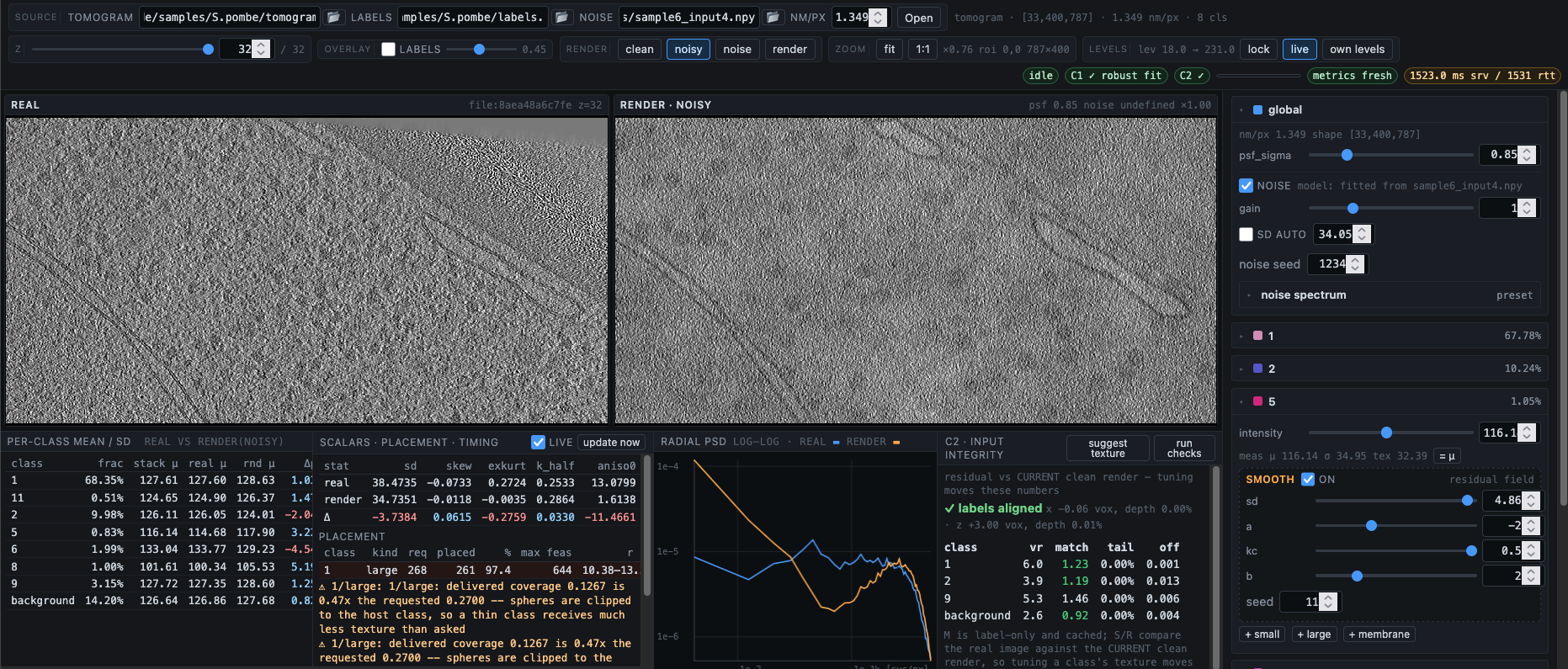The workbench: file inputs, per-class controls, live clean/noisy renders, and the metrics panel

Starting It

cd renderer_code
python tuner_server.py --port 8765
# open http://127.0.0.1:8765/

A small local web app: a standard-library HTTP server (tuner_server.py) serves a single-page UI (tuner.html) and drives the render engine (render_layers.py). File paths are read server-side — they are paths on the machine running the server.

Opening a Source

Fill the top bar and press Open:

Field	Requirement
tomogram	.tif/.tiff, .mrc, or .npy intensity stack
labels	Same shape as the tomogram; integer labels, 0 = background
noise	A noise-model JSON, or a clean background-crop stack (.tif/.mrc/.npy)
nm/px	Pixel size in nanometres

When you give a crop instead of a JSON, the workbench fits the noise model server-side (spectrum + banding + axial; reduced budget, ~2–3 min the first time), runs the C1 cleanliness checks on the crop, caches the result as <crop>.noisefit.json next to the crop (instant on re-open; delete the sidecar to refit), and reports the verdict in the C1 badge. A pasted production-fit JSON always wins over fitting.

What You Tune

For each label class, the workbench measures the class's grey mean/sd from the tomogram, then gives you:

• Object populations — small blobs with adjustable coverage, contrast, size (in nm), and clustering. Populations start empty; you build them up per class. Placement is non-overlapping and deterministic.
• A smooth per-class field — low-frequency intensity variation inside the class.
• A membrane band — a border of declared thickness (nm) and contrast where the class touches its neighbours (all, or a named subset), geometry derived from the labels.

Then a PSF is applied, and noise from the model is stamped at the model's amplitude. The clean and noisy renders update live as you drag controls.

The Metrics Panel

Per-class statistics and spectral descriptors of the real vs rendered image, computed by the same noise_metrics.py the validation uses — so what you see while tuning is what the scorecard will measure.

C2: Input Integrity

The "C2 · input integrity" panel (/api/validate) runs the input checks of the corruption study:

Test	Detects
M	Label misalignment (shift recovery, sub-voxel)
S	Leftover structure in the background vs a mask-matched null
R	Per-class mean residual in noise-sd units

Run it before investing tuning time — a misaligned label stack quietly corrupts every class measurement.

Saving and Loading Configs

Save writes a config JSON (per volume, one render config: source, nm_per_px, psf_sigma, noise{...}, classes{...}). Load applies a saved config to the currently open source — open the matching files first.

The HTTP API

Everything the UI does is a JSON call, scriptable directly:

Endpoint	Purpose
POST /api/open	{image, labels, noise, nm_per_px} → source handle, shape, measured classes, default config
POST /api/render	{source, config, z, roi?, want?, want_metrics?} → PNG panels (+ metrics)
POST /api/save / GET /api/load?name=	Config persistence
POST /api/validate	{source} → the C2 checks

A source handle stays valid while the server runs; after a restart, press Open again.

Notes

• The label stack must segment the same volume as the tomogram (same shape) — intensities are read per label from the tomogram.
• Real structure inside a class is captured as its mean and spread; the object populations you add are the tunable texture on top.
• .mrc input needs mrcfile; everything else is numpy/scipy/tifffile/matplotlib.

Related

• Tutorial: tune your own volume — the full workflow with quality gates
• The Noise Model — what the noise file contains